Music Scores is a puzzle that both fascinated and intimidated me. On the one hand, learning about image processing and pattern recognition could be very cool; on the other, it seemed incredibly hard.
How could I possibly solve it?
After carefully analyzing the problem, I could see how much it could be simplified. I realized the puzzle might not require high-level coding knowledge after all!
Disclaimer: The following is a simple outline of how you might try to solve the Music Scores puzzle. I’m proposing my analysis of it, but I’m sure you can come up with more optimized ways to solve it.
Primary Analysis
The goal of the puzzle is to decode an image representing a music score.
This is what we know:
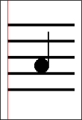
- A musical staff contains 5 black lines
- Notes lie either between 2 lines, or on a line
- All 5 lines have the same height
- The spaces between the lines (I will be calling it note height) are all uniform
- Half notes will have at least one white pixel within the circle
Interpreting the Grid
The image is given encoded with a simple form of Run-Length Encoding (RLE), a fancy term meaning consecutive pixels of the same color are grouped together and termed as “color number_of_pixels.”
Example: “B 4 W 7” is decoded to 4 black pixels followed by 7 white pixels.
We store the grid in a boolean w*h grid (where w, the width of the maze and h, the height of the maze, are given to us). The RLE version of the image starts from (0,0) and runs horizontally from left to right (wrapping onto the next line below, not always explicitly). It is preferable to store black pixels as true, as they are fewer in number.
Let’s read the RLE code and track the current x and y value, initially set to (0,0). If a white set of pixels is given, just update x and y accordingly without making any changes to the grid. When a black set of pixels is given, run a loop for the number of pixels, incrementing x value by 1 every time, and setting grid[x][y] as true. No need to worry about wrapping, as no image has a line ending with a black pixel.
And we’re set! There are more functionalities defined in this interpretation loop in the final solution, but I’ll go over them later.
Locating the Lines
In my opinion, locating the lines is our foremost concern, as rules help us detect the notes.
Now for our first step into image processing: How do we know where a line starts?
At first, I thought that the first black pixel I encountered while interpreting the grid was the start of the higher line. Not necessarily, though, as the tail of a note could go above the higher line and contain that first black pixel.
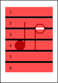
So what, then? I noticed that the leftmost black pixel always belonged to a line. THIS could be calculated. How? We keep a minx and miny value while filling the grid. Whenever we encounter a black pixel, if its x value is less than minx, update it and set the current y value to miny.
Now we have the x-position of the red line in the figure above, defined by x = xmin. What next? We know that all lines have equal height. So if we count all the black pixels on this red line and divide by 5, we have the line height (lineH).
Sweet! Let’s find the note height (noteH) now. It’s the same as the space between two lines. We can calculate this by counting the number of pixels between minY+lineH and the next black pixel below, still on the red line of course. There are more optimized ways of doing this, but I will not be discussing them here (hint: something to do with the total number of white pixels between the first and last line).
So we have located all the lines. Now, you might wonder why we did all calculations with this particular red line. We could simply do it with the line defined by x = w/2, which will always cross the staff, couldn’t we? Well, there is no guarantee that at x = w/2, we won’t also find a note. Whereas at the red line, i.e., where we could find the black pixel that is farthest to the left, there will never be a note present.
The code to locate the lines can be included in the grid-interpretation loop.
Vertical Zonal Marking
My algorithm should roughly detect the center of a note. Once we know the position of the lines, estimating the type of note (half or quarter), given its y value (its label), should not be too hard. So let’s divide the entire staff into 12 sections, each section holding a particular type of note.
Note that the division will vary depending on which part of the note we are detecting first. In our case, it is the center of the note, y-axis wise.
In the pseudo-code given below, observe the use of sum and lnt. Sum stores the total height of a line + space. lnt is half of sum. This is helpful as we divide these spaces into equal halves (as per the diagram).
Notice that, since we are halving noteH + ruleH, the center of a note falls clearly within a zone, and there is no edge condition (i.e., the center of a note does not fall on the separation of 2 zones):
void init() {
  int sum = noteH+lineH;
  int lnt = sum/2;
  zone[0] = new Zone(minY,minY+lnt);
  zone[1] = new Zone(minY+lnt,minY+sum);
  zone[2] = new Zone(minY+sum,minY+sum+lnt);
  zone[3] = new Zone(minY+sum+lnt,minY+sum*2);
  zone[4] = new Zone(minY+sum*2,minY+sum*2+lnt);
  zone[5] = new Zone(minY+sum*2+lnt,minY+sum*3);
  zone[6] = new Zone(minY+sum*3,minY+sum*3+lnt);
  zone[7] = new Zone(minY+sum*3+lnt,minY+sum*4);
  zone[8] = new Zone(minY+sum*4,minY+sum*4+lnt);
  zone[9] = new Zone(minY+sum*4+lnt,minY+sum*5);
  zone[10] = new Zone(minY+sum*5,minY+sum*5+lnt);
  zone[11] = new Zone(minY+sum*5+lnt,minY+sum*6);
}
Locating the Notes
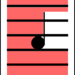
We will be sweeping across the white spaces between rules.
If we find a black pixel in here, it surely belongs to a note. The 6 regions we sweep across are shown in the picture. Now, sweeping can be done in 2 ways: horizontally and vertically. Let’s take a look at the pros and cons of each of these sweeping techniques.
Horizontal Sweep
A horizontal sweep iterates over pixel rows, from the left to the right and from the top to the bottom.
I say this is HIGHLY disadvantageous.
- If we stop at the first black pixel in each line, we can’t be sure we’ve found the first note of the staff. We could reorder the notes afterwards, but this just makes it more complex.
- Differentiating the tail from the circle of a note with code isn’t as straightforward as it might seem. Sure, we know when and where a tail goes up or down and when it is on the left or on the right of the circle. But if a tail is encountered first, gauging the position of the note will be quite hard.
(We could create another zonal marking system for the tail, too, but tails will not always be encountered first, and again this results in the same problem – differentiating the tail from the circle.)
I have only stated 2 disadvantages; how does that make it “highly” disadvantageous? Simply the fact that there are no particular advantages stated. Let’s see why a vertical sweep is a much better choice.
Vertical Sweep
I think my choice was fairly clear in my criticism of the horizontal sweep. Here, I propose to analyze each pixel column one after the other, from the top to the bottom and starting from the left.
I prefer it because:
- It makes us analyze one note at a time, in the right order.
- An upward tail never comes before the note, so we always encounter the leftmost pixel of the circle FIRST.
- The position of the note can be easily calculated as the distance between the first column with an anomaly and the next column without any.
Now that the choice is made, let’s proceed with the algorithm again.
The Algorithm
We perform a vertical sweep from the top to the bottom, from x = minx to maxx. We should ignore the staff lines.
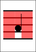
Let’s suppose we encounter a black pixel. We store the x and y position of this pixel, say as refx and refy. We now have a note. We continue sweeping until we reach a column without an anomaly (with no unknown black pixel). Say this x-position is refx2. Now let’s check the color of the pixel at the center of the segment between these two references (refx, refy) and (refx2, refy). This is near the center of the note circle. For a half note it should be white, and for a quarter note it should be black. We can now add the suffix Q or H.
Next we use the zonal marking system to get the note type by passing refy as the argument. These are the notes which the zones stand for:
switch (position) {
  case 0: add = "G"; break;
  case 1: add = "F"; break;
  case 2: add = "E"; break;
  case 3: add = "D"; break;
  case 4: add = "C"; break;
  case 5: add = "B"; break;
  case 6: add = "A"; break;
  case 7: add = "G"; break;
  case 8: add = "F"; break;
  case 9: add = "E"; break;
  case 10: add = "D"; break;
  case 11: add = "C"; break;
}
Yaay! We now have both the note type and the suffix! Continue sweeping till the end of the staff to detect all the notes, AND WE ARE DONE!!! ^_^
Conclusion
Well, that’s it! We can now locate notes and determine their type on a music score. The only possible bug that comes to my mind is the following: If you are not sweeping exactly between lines and your algorithm detects a line and takes it as a note, all is ruined. So yes, make sure to go exactly between the lines!