Hello, folks. I’m Vlado, from Bulgaria. I’m a big fan of CodinGame, and I really try to improve my programming skills every day.
I joined CodinGame 3 years ago and immediately felt that this would be the best place to practice my coding. At first, I started participating in contests. But after a few of them, I realized I had to practice more to get better results.
I joined online courses on AI and Algorithms topics. I also started to ask questions in the CodinGame chat; there, MadKnight gave me many useful tips. At first, I didn’t think the Practice section was very good for training. But now I’m very excited and proud of myself every time I earn an achievement.
The biggest challenge, so far, has been the Mars Lander puzzle (all 3 episodes). I really liked the task, because it could be solved with Genetic Algorithm (GA).
Genetic Algorithms on CodinGame
GAs are often used on CodinGame. Some top contest players have already written in the forum or on the blog how they used GAs to get the leading positions in a contest. So I thought exercising GA would help me get better and maybe even open the doors to Neural Networks.
I was determined to solve the task using GA and C++ as a language. Of course, there are other ways to solve it; for example, with a pure physics approach. This approach is fine, but from the solutions I saw, there is a fair amount of hardcoding, which I’m not sure will work well in all environments (other tests than the given for the puzzles). The GA gives you a solution, if one exists, for every possible case.
Simulation
A good GA requires a good simulation for the Lander: moving it based on the rotation, thrust and current speed. I would know my simulation algorithm would work if, from a set of rotation and thrust commands, I could get the same results as the ones from the CodinGame simulator.
I first tried a naive approach, but couldn’t get it to work correctly, despite several iterations. I was sure there was something in the physics I didn’t understand. I needed to clarify the physics behind the problem, so I could feel comfortable with my simulation algorithm. To do that, I went through almost all motion physics learned in school, from this site: physicsclassroom.com.
It took me several days. But, at the end, I had a smooth, working simulation.
Chromosomes, Genes and Population
The next step was to come up with a good representation of the algorithm components. I needed to decide how to store information for Chromosomes (individuals) and their Genes in a Population. This representation is the base of your algorithm, so if it is not solid, your algorithm will fail.
At first, I chose to use the Standard Template Library (STL). The Gene class contained only two members: rotate and power, representing the rotation angle and the thrust power for the Lander. A Chromosome was a vector of Genes. And the Population was a vector of Chromosomes:
class Gene {
public: …
private:
  int rotate;
  int power;
};

typedef vector<Gene> Chromosome;
typedef vector<Chromosome> Population;

class GeneticPopulation {
public: ...
private:
  Population population;
};
Pretty simple and intuitive, right? 🙂
Once I had chosen the representation, I needed to define the first population, also known as Initial Random Population. I began with 40 chromosomes, with 40 genes each. That gives me 1600 genes, for which I generated random rotations and powers. I used a [90, -90] range for the rotation and a [0, 4] range for the power. When simulating, I clamped the rotation and power to be in the allowed range, based on the previous move.
I was wondering if 40 genes were enough for the simulation, if the initial population was good, if it was well distributed…I quickly realized that no matter how much I debug and write down things, I couldn’t answer those questions properly. I desperately needed some way to visualize the data, so I started writing my own debug tool.
Visualization
I began with OpenGL, but couldn’t find a tool that worked well enough for my purpose. So I ended up writing a visual debug tool using JavaScript and SVG. I dump the information for all paths formed from commands in the chromosomes’ genes starting from the initial Lander position. Then the tool writes that information in SVG polylines in an html file, which can be easily viewed in a browser:
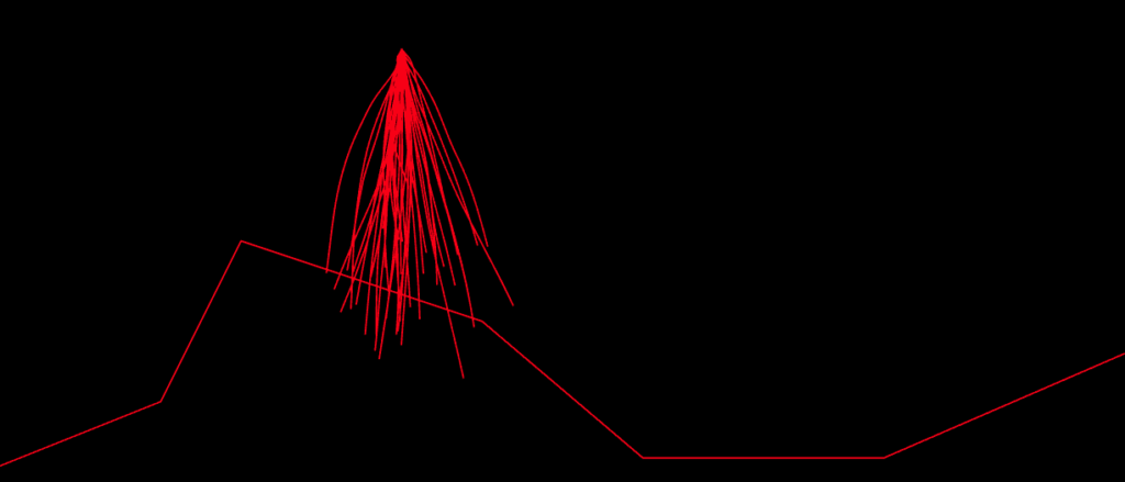
Here, each strand represents a path for the Lander, from its initial position, using the commands of the corresponding chromosome.
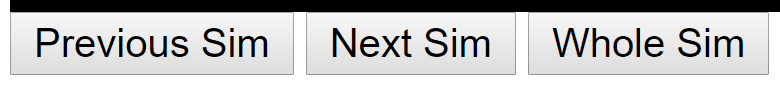
Later, I added some buttons (and shortcuts) to play the whole simulation and navigate through each iteration of the population:
For convenience, I implemented a popup, which shows the properties of the Lander (after the whole simulation of the chromosome), as soon as the mouse hovers over a path:
This visual tool took me several weeks to complete. I’m very satisfied with the result.
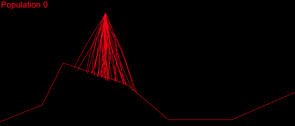
Instantly, I noticed several things. The initial paths were too short and too close to each other. They didn’t spread very wide above the Mars surface and there were too few of them. I would never have realized that without a visual debugging.
The narrowness between the paths was due to the random ranges [-90, 90] and [0, 4] for rotation and power respectively. I often generated values far beyond the restrictions, and when clamped, for the simulation process, chromosomes were filled with 15s and 0s. For example, the random generated rotation angles are: [90, 64, 82, …] and this means Lander rotations (clamped) are [0, 15, 30, …]; each rotation is with the maximum step, for a turn – and this was very often.
So I decided to generate random numbers in the [-15, 15] and [-1, 1] ranges and, at each iteration, add them up to the previous values. This way I got more scattered random angles and the paths spread more widely. I also increased the Chromosome size to 60:
Collision vs Landing
A very important thing was to decide how to check if the Lander collides with the ground. At each simulation (for a given chromosome), every time I apply a command, I store the current and previous positions of the Lander, which form a line. Then, I check to see if that line intersects a line from the surface. If there is an intersection, I stop the simulation.
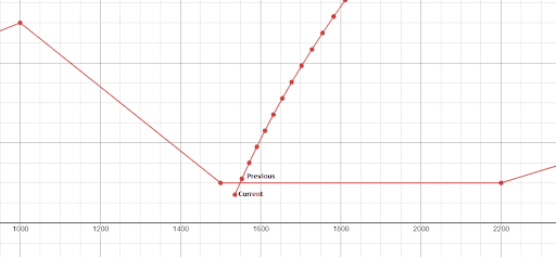
I also wrote a function which checks if the Lander is good for landing. If the Lander path intersects the landing zone, and both states (before and after the line) of the Lander are within satisfactory properties (speed and rotation in range [-15,15]), we’ve got a solution. So the only thing left is to update the rotation command stored in the gene for Previous state to be 0 (and keep the thrust power, preventing the Lander from going up or increasing its down speed) so it can land in vertical position.
Evaluation Function
Once the simulation is done, the next step is to come up with a good evaluation function. It took me a dozen tries to realize the most important things:
- the distance from the crash to the landing zone
- if the Lander crashes on the landing zone, high speeds and big angles should be considered as disadvantages.
Genetic Modifications
The first tutorial I took on GA was the one by Sablier. From there, the plan was to implement 3 main operators:
- Selection
- Crossover
- Mutation
For the selection, I used the Roulette wheel selection method. It involves normalization, sorting and cumulative summing of the values (as calculated by the evaluation function) of each chromosome. An example will be worth a thousand words:
| Chromosome 0 | Chromosome 1 | Chromosome 2 | Chromosome 3 |
| 83.5 | 10 | 120.2 | 33.3 |
The sum of all evaluations is 247. To normalize, divide each evaluation with the sum:
| Chromosome 0 | Chromosome 1 | Chromosome 2 | Chromosome 3 |
| 0.338 | 0.04 | 0.487 | 0.135 |
Sorting the chromosomes in descending order:
| Chromosome 2 | Chromosome 0 | Chromosome 3 | Chromosome 1 |
| 0.487 | 0.338 | 0.135 | 0.04 |
Calculating the cumulative sum:
Chromosome 2 = Chromosome 2 + Chromosome 0 + Chromosome 3 + Chromosome 1
Chromosome 0 = Chromosome 0 + Chromosome 3 + Chromosome 1
Chromosome 3 = Chromosome 3 + Chromosome 1
Chromosome 1 = Chromosome 1
| Chromosome 2 | Chromosome 0 | Chromosome 3 | Chromosome 1 |
| 1.0 | 0.513 | 0.139 | 0.04 |
The Roulette wheel selection works by choosing a random number between 0 and 1 and selecting the first chromosome having a computed value greater than this number. Every time a selection is performed, two different parent chromosomes are chosen to make two children. In this example, if the random number is 0.8, we choose Chromosome 2, then a new random number is generated, for example 0.1, and the second parent is Chromosome 3 (choosing a second parent is repeated until the chosen chromosome is different from the first parent). This selection is used every time we need to do a crossover of chromosomes.
My first try for a crossover was to split the two selected chromosomes (parents) at a random index:
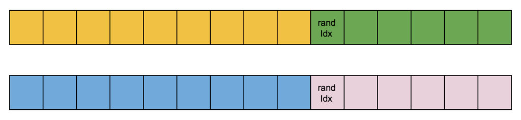
And make new chromosomes by recombining parents’ split parts:
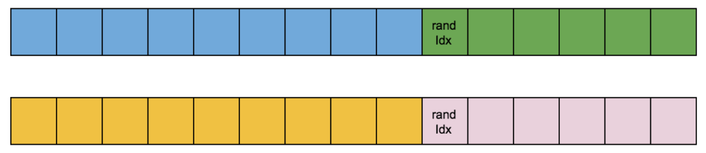
For the mutation, I changed one gene in every new chromosome with a random one:
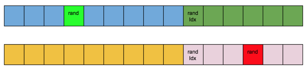
I repeated the process until my new population reached the size of the current one. For example, if the population size was 40, I selected pair of parents 20 times and performed 20 crossovers to produce 40 children. This is how it’s done in most of the GA tutorials I watched.
Testing
After fixing a ton of bugs, this is how my first simulation with 200 populations looked:
It took a couple of months to get there. But I wasn’t satisfied. My algorithm was slow, it didn’t cover a large enough part of the search space and was quite far from converging. I played with the algorithm variables as much as I could:
Still nothing. Apparently, I had missed something.
At that time, I just wanted to find a solution for one of the easiest tests “Easy on the right.” Just a single set of commands, which would land my Lander in a safe position: not the optimal, nor the fastest. But whatever I tried didn’t help; I was watching my algorithm fail to converge over and over again.
I knew that I didn’t need that many populations. So, I decided to enroll in an online course on GA to get deeper knowledge in the field and hopefully find out what I was missing.
Continuous Genetic Algorithm
There I learned the term Continuous Genetic Algorithm. This means that, when your chromosome representation is not only with bits, but with real numbers (which is my case), there is a better way to crossover and mutate the chromosomes. This leads to a better transversal exploration of the search space and better children in the next generation.
The crossover becomes a weighted sum of two chromosomes using a random number between 0 and 1:
child0Gene[i] = random * parent0Gene[i] + (1 – random) * parent1Gene[i];
child1Gene[i] = (1 – random) * parent0Gene[i] + random * parent1Gene[i];
For example, if our random number is 0.8:
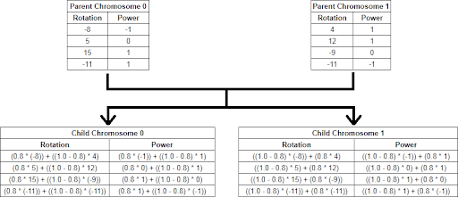
In this type of GA, each gene of the child chromosome has a chance to mutate. Again, I used random numbers between 0 and 1, and checked them against a specific constant (the Probability of Mutation). This way, there was a bigger chance to explore a large part of the search space. However, be careful: big mutations may lead to a random search, which won’t converge in a century. At the end, I chose a Probability of Mutation of 0.01.
One of the most important things I found is that using elitism helps the algorithm a lot. This means to copy the best chromosomes from the current population directly into the new population. I found that copying 10% to 20% of the chromosomes works nicely.
After a lot of polishing and debugging, I finally saw the end of it: a real convergence of my algorithm – and a solution!
This was truly awesome. I couldn’t believe my eyes. The work finally paid off.
I tried the other tests in the puzzles and they all worked. Then I thought: Why not try “Cave, wrong side,” – the hardest test in episode 3? I was absolutely sure it wouldn’t work; my collision detection was not perfect, maybe had some random issues, but ……..
LOOOOOOOOOOOOOOOOOL IT WORKED……! I almost couldn’t sleep that night!
Time Constraints
The time had come for me to migrate my algorithm to CodinGame. First of all, it had to respect the time constraints. My initial idea was to run the whole algorithm during the first turn, generate the solution chromosome and issue a command for each of its genes at every turn: fifth turn – fifth gene from the solution. I measured the time needed for my algorithm on each test case and it wasn’t good at all. For the “Initial speed, wrong side” test, my algorithm needed several minutes. There I had my algorithm converge after 400 populations:
My goal was to get in the time frame for the first turn, and this meant to calculate 400 populations in several seconds. I knew I could do that.
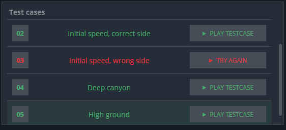
I started by separating my code for the visual debug tool from the algorithm code. This wasn’t smooth and easy and took me a couple of days. Then, most of the tests passed, but the “Initial speed, wrong side” test didn’t:
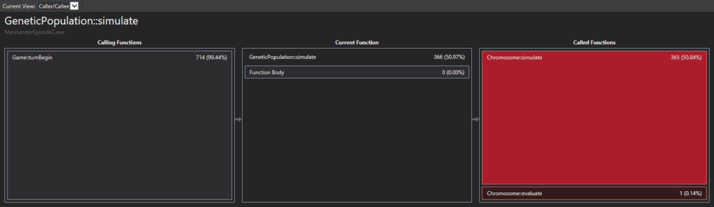
I tried simple tweaks and tricks, but I didn’t get much improvement. I then realized that I had to use some kind of profiler. I chose the Visual Studio one: simple and intuitive. It shows the biggest bottlenecks with big red rectangles, which usually are functions. You can select the rectangle and step in the function to see what is causing the delay:
The first thing I saw was the really large amount of time swallowed up by the STL. Internally, the STL structures are invoking many new and delete operations, which consumes a lot of time. I used the STL to represent my population, using many vectors and maps. This was surely slowing my algorithm. I decided to stop using the STL. The best representation I thought of was the following:
const int CHROMOSOME_SIZE = 100;
const int POPULATION_SIZE = 100;

class Gene {
public: …
private:
  int rotate;
  int power;
};

class Chromosome {
public: …
private:
  Gene chromosome[CHROMOSOME_SIZE];
};

class GeneticPopulation {
public: ...
private:
  Chromosome populationA[POPULATION_SIZE];
  Chromosome populationB[POPULATION_SIZE];

  Chromosome* population;
  Chromosome* newPopulation;
};
The Chromosomes are represented as basic C++ arrays. And I have pointers to the current and the new populations. All operations on the populations are made through these pointers. First, the population pointer points to populationA, which contains Initial Random Population. newPopulation points to populationB. When a crossover is performed, the new children are written in the array through the newPopulation pointer. After mutation and elitism are performed, I switch the pointers for the population arrays:
// Switch population arrays
if (0 == (populationId % 2)) {
  population = populationB;
  newPopulation = populationA;
}
else {
  population = populationA;
  newPopulation = populationB;
}
When new children are created, I overwrite the ones in the previous generation. That was the biggest optimization in my code.
One other big thing was the preparation of the Roulette Wheel. At first I had 4 main steps, each involving a complete iteration of the entire population:
- A loop to sum the value of all chromosomes
- A loop to normalize the value of all chromosomes
- A sorting of the chromosomes
- Two nested for loops to calculate the cumulative values
I combined all those steps into one. I used a member in the population to hold the sum of all values. Every time I evaluated a chromosome, I would add its value to the sum. Next, I added std::map<float, int> chromEvalIdxPairs (STL, but this time worth it) to store chromosome value and chromosome index pair.
Now, when preparing chromosomes for the Roulette Wheel, I had one for loop iterating the population, normalizing the values and adding them to the map. The main trade-off was that the sorting step (which was very slow) was skipped, because when iterating std::map, the elements are iterated in sorted order ;). I left the calculation of accumulated values to the selection step. So my selection looked like this:
float r = Math::randomFloatBetween0and1();

float cumulativeSum = 0.f;
parent0Idx = chromEvalIdxPairs.rbegin()->second;
for ( ChromEvalIdxMap::const_iterator it = chromEvalIdxPairs.begin();
    it != chromEvalIdxPairs.end();
    ++it
) {
  cumulativeSum += it->first;
  parent0Idx = it->second;

  if (r < cumulativeSum) {
    break;
  }
}
And keep in mind that map::const_reverse_iterator is way slower than map::const_iterator! I learned that the hard way!
Finally, I found that my algorithm needed 200 genes per chromosome to pass the “Cave, wrong side” test rather than 100 genes like the other tests.
These optimizations were enough to pass all the tests:

I couldn’t stop there, though! I wanted to investigate other solutions and to really see what my algorithm was capable of. I wanted to solve more complex tests without any time limit, so I grabbed the one from the tech.io tutorial. There, 200 chromosomes, with 300 genes each, were needed in each population and above 1000 populations:
Here displaying every 10th population.
I learned a lot from this puzzle! I was determined to solve the task, and no matter how much time I spent, I never quit – I just kept improving what I had. The main lessons I learned from this experience are: Keep it simple, no need for fancy complicated stuff, and, most of all, NEVER stop believing.
Cheers,
Vlado